Deep dive on logits in neural networks

I used to be afraid of logits. I thought ML models' outputs were labels or numbers - so what's the deal?

The concept was both scary and confusing to appoarch for me for the longest time. The search space for hyperparamaters is non-trivial and thus a struggling ML student gotta prioritize! Eventually, as a visual learner I eventually came upon a way to help wrap my head around what logits are, and by extension, CE loss. Understanding what logits are also helped me understand how to effectively select the correct loss function for the task. This blog post documents my own way to understanding logits - and hopefully, would also be of use to you!

What Exactly Are Logits?

For models doing classification tasks (let's call them cls_head(s),) a neural network's final layer produces raw, unnormalized scores for each class. These scores are logits, and most often they are immediately processed again into a label (by first dividing by temp, optional) and then softmax, and then either argmax or multinomial pick from this distribution. Was that TMI? Think of logit as the model's "confidence" score for each label. A higher logit means the model is more confident in that class being the correct one.

Raw logits have a couple of limitations:

• They are not easily interpretable. They're semi-arbitrary. For example, while both model A and model B may output the same label 1, perhaps label 1 was scored a 10 by A but 900 by B. .
• Logits can be any real number, from negative infinity to positive infinity depending on your activation function at the last layer.

Logits in Binary and Multinomial Classification

The concept of logits is central to both binary and multinomial classification problems:

• In binary classification, the model typically outputs a single logit. A positive logit suggests one class, while a negative logit suggests the other. You can indeed make the model output a logit for each class, but that's just unneeded extra compute.
• In multinomial classification, the model outputs a vector of logits - one logit for each possible class. The class with the highest logit is the model's prediction. But wait - wasn't logits semi-arbitrary?

Standardizing Logits into Probabilities: The Softmax Function

To make logits more interpretable, we need to convert them into probabilities. This is where the softmax function comes in. Basically, we are normalizing a vector of logit scores into values between [0, 1]. This essentially yields a probability distribution, where:

• Each value is in [0,1].
• They all sum up to 1.

Here's softmax (each z is each label's logit - so if your last layer is 3 nodes for a 3 label cls head, it's [z1, z2, z3]):

$$ \text{softmax}(z_i) = \frac{e^{z_i}}{\sum_{j=1}^{K} e^{z_j}} $$

As you see, doing exp() biases for positive logits as they will explosively grow, while exp() will drop to 1 as logits hits 0, and approaches 0 as logits goes to -inf. The point is, all outputs are now converted into positive values, and by nomarlizing them all by dividing by sum - they get between [0,1]. Great - now we have manufactured a way to bias for outputting highest logit values for correct labels - after a couple epochs with backprop we can fully expect the model to output the highest logit score for correct y (note that this is also the only expectations we can have, as model behavior for the other y labels can be chaotically anywhere between assigning them -inf or -1, as long as the correct y is the highest value.) This direction thus has its own biases, but it does the job and it can be implemented with NLL.

Calculating the Loss: Log and Negative Log-Likelihood (NLL)

We have "probabilities" which is interpretable as the model's confidence on each label to assign. We have them softmax so they all fall neatly in [0, 1] distribution. However, we still need some further steps to meet 2 limitations. One is that the convention for training in deep learning is to minimize loss, not maximizing correctness - so a simple invertion is needed. Two is runtime complexity: arithmetic operations linearly scales with the number of decimal places (fewer bits to do math on .1 versus .00...001) - so a little trick to apply log to the softmax values is needed to take us out of this sink hole of decimal points. This is pretty relevant for cls head/models dealing with multinomial labeling from a pool of tens of thousands labels - i.e. a LLM model operating with the vocabulary size of languages!

So ok, now we need to eval our model. We need a loss that tells the model not just if it was wrong, but how wrong it was. This function needs to do two things: turn "maximizing correctness" into a "minimizing loss", and handle the softmax values in a way that use as few binary bits as possible.

So now we do NLL: $$ \mathcal{L}_{\text{NLL}} = -\log(p_{c}) $$

In this formula, p_c is the softmax probability for the one correct class, c. Note that indeed, NLL doesn't care at all about the softmaxed values of other labels by design (other loss like KL would - not NLL.) Let's unpack why this simple formula is so effective:

• The log function acts like a magnifying glass for probabilities. It transforms the cramped [0, 1] space into a sprawling [−∞, 0] space, making differences between small numbers (like 0.01 vs 0.001) much larger and more numerically stable for the computer. (i.e. instead of 0.0001 * 0.001, which uses floating point representation and risks underflow, we can do its mathematicaly equivalent of log(0.0001) + log(0.001), which is simply -9.2 + (-6.9) = -16.1)
• The negative sign flips this range to [0, ∞). Now, a perfect prediction (probability 1) gives a loss of -log(1) = 0. A terrible prediction (probability close to 0) gives a huge loss. We now have a "cost" that our model can try to minimize.

The Wrapper Module: Cross-Entropy Loss

In practice, you'll hear about CE Loss but almost never softmax or NLL. In truth, CE Loss is basically softmax + NLL. $$ \mathcal{L}_{\text{CE}} = - \sum_{i=1}^{K} y_i \log(p_i) $$

This formula looks more complex, but it's doing the exact same thing. Here, y is the "ground truth" vector, which we represent with one-hot encoding. For example, if the second of three classes is the correct one, then y = [0, 1, 0]. The vector p holds our model's predicted softmax probabilities.

When you compute the sum, every term where the true label y_i is 0 gets zeroed out. The only term that survives is the one where y_i = 1. Nice, so CE loss collapses down to NLL, -log(p_c).

Now, for the Gradient:

So, we have a loss value. Now what? We need to backprop that single number into millions of tiny nudges for each weight and biases in our neural network. With a bit of chain rule, we get the the derivative (or gradient) of the loss with respect to every parameter.

Visualizing: Epoch 5 vs. Epoch 45

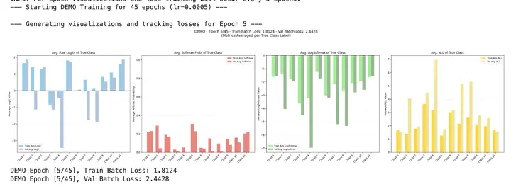
To see how these values evolve during training, let's look at a couple of snapshots. First graph is raw logit, 2nd is softmax, 3rd is log of softmax, and 4th is the negative of that log (NLL).

Epoch 5

In the early stages of training, the model is still learning. The average softmax of correct label is still <.4, and after NLL we get 1.8 loss which is relatively high. We also include a validation set results in these charts for a sense of the model underperforming on both partitions in the beginning.

Epoch 45

After more training, the model has learned to distinguish between the classes better in the training samples. Notice how the model is outputting nearly .8 softmax for the correct label! Recall that the final label is retrieved using argmax or multinomial pick, so anything that makes a label a "majority vote" is already sufficient. NLL in the training set has now been pushed down to near 0! Sadly, note that validation set NLL spiked - representing overfit.

So what?

So CE Loss did its job: it has now tuned the model to output the highest possible logit score for the correct label in the training set. The model is now akin to a route-memory parrot where it can assert with high confidence what the correct answer is to be for any samples it has seen thanks to CE Loss. However, it failed to converge towards generalizability - representing the need for other hyperparameters and mechanisms to further improve our model. That's a story for another day as we now have a grasp of how logits work!

Conclusion

Understanding logits is key to understanding how classification models work. They are the raw output of the model, which, when passed through the softmax function, can be interpreted as probabilities. By then calculating the negative log-likelihood, we get a loss value that we can use to train our model. As we've seen, the values of the logits, softmax probabilities, and loss all change as the model learns, reflecting its increasing confidence and accuracy.

We hope this post has helped you better understand the role of logits in neural networks. Thanks for reading!

---